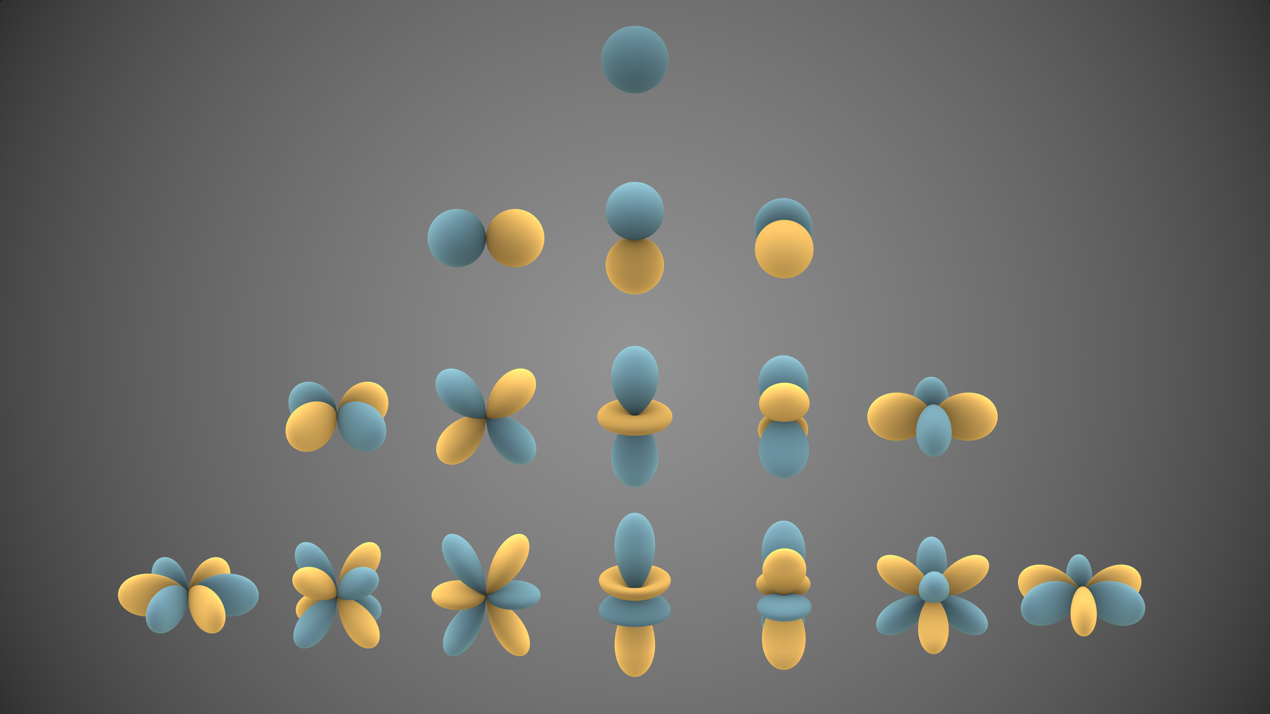
Solving the rigid rotor Schrödinger equation leads to a special class of angular wavefunctions known as spherical harmonics. These functions describe the allowed angular distributions of a rotating molecule and are the simultaneous eigenfunctions of the rigid rotor Hamiltonian and the angular momentum operators.
Because the rigid rotor has no radial motion, its wavefunctions depend only on the angular coordinates \(\theta\) and \(\phi\). The solutions therefore take the general form
\[ \psi(\theta,\phi) = Y_\ell^{m_\ell}(\theta,\phi), \]
where \(\ell\) and \(m_\ell\) are integers that arise from the separation of variables.
Structure of the spherical harmonics
The spherical harmonics are constructed directly from the separated angular solutions:
- a polar-angle function that depends on \(\theta\),
- an azimuthal-angle function that depends on \(\phi\).
Explicitly, each spherical harmonic can be written as
\[ Y_\ell^{m_\ell}(\theta,\phi) = N_{\ell m_\ell}\, P_\ell^{m_\ell}(\cos\theta)\, e^{i m_\ell \phi}, \]
where:
- \(P_\ell^{m_\ell}(\cos\theta)\) are the associated Legendre polynomials,
- \(e^{i m_\ell \phi}\) describes rotation about the \(z\)-axis,
- \(N_{\ell m_\ell}\) is a normalization constant.
The appearance of the associated Legendre polynomials reflects the solution of the \(\theta\)-equation, while the complex exponential reflects the solution of the \(\phi\)-equation.
Legendre and associated Legendre polynomials
The angular equation for the rigid rotor leads to a family of special functions known as Legendre polynomials and associated Legendre polynomials. These functions arise naturally when solving differential equations that depend on the polar angle \(\theta\).
Legendre polynomials
When the separation constant \(m_\ell = 0\), the \(\theta\)-equation reduces to the Legendre differential equation. Its solutions are the Legendre polynomials, denoted \(P_\ell(x)\), where \(x = \cos\theta\).
The integer \( \ell = 0,1,2,\ldots \) labels the order of the polynomial. Each \(P_\ell(x)\) is a polynomial of degree \(\ell\).
The first few Legendre polynomials are:
\[ \begin{aligned} P_0(x) &= 1, \\ P_1(x) &= x, \\ P_2(x) &= \tfrac{1}{2}(3x^2 - 1), \\ P_3(x) &= \tfrac{1}{2}(5x^3 - 3x). \end{aligned} \]
These functions are orthogonal on the interval \(-1 \le x \le 1\) (equivalently \(0 \le \theta \le \pi\)), reflecting the orthogonality of different angular momentum states.
Associated Legendre polynomials
For nonzero \(m_\ell\), the solutions of the \(\theta\)-equation involve the associated Legendre polynomials, denoted \(P_\ell^{m_\ell}(x)\).
These functions are obtained from the Legendre polynomials by differentiation:
\[ P_\ell^{m_\ell}(x) = (1-x^2)^{m_\ell/2} \frac{d^{m_\ell}}{dx^{m_\ell}} P_\ell(x), \qquad m_\ell \ge 0. \]
The associated Legendre polynomials are defined only for integer values satisfying
\[ |m_\ell| \le \ell. \]
This restriction ensures that the solutions remain finite at \(\theta = 0\) and \(\theta = \pi\).
Physical interpretation
The Legendre polynomials describe the angular dependence of states with zero projection of angular momentum along the \(z\)-axis (\(m_\ell = 0\)).
The associated Legendre polynomials describe how this angular dependence is modified when there is a nonzero projection of angular momentum (\(m_\ell \neq 0\)).
Together with the azimuthal factor \(e^{i m_\ell \phi}\), these functions form the mathematical foundation of the spherical harmonics.
Big idea: Legendre and associated Legendre polynomials encode the polar-angle dependence of rotational wavefunctions and serve as the essential building blocks of the spherical harmonics.
Quantum numbers and allowed values
The integers \(\ell\) and \(m_\ell\) are constrained by the requirement that the wavefunction be finite and single-valued:
\[ \ell = 0,1,2,\ldots, \qquad m_\ell = -\ell, -\ell+1, \ldots, \ell. \]
Each value of \(\ell\) corresponds to \(2\ell+1\) degenerate spherical harmonics with different values of \(m_\ell\).
Big idea: the spherical harmonics provide a complete, orthonormal set of angular wavefunctions for rotational motion. They are built from Legendre and associated Legendre polynomials and encode the quantized angular structure of the rigid rotor.