
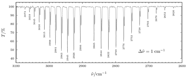
In real molecular spectra, vibrational and rotational motions are often observed simultaneously. Such spectra are known as rotation–vibration spectra. A classic example is the \(v=1\leftarrow 0\) infrared band of HCl near \(2990\ \text{cm}^{-1}\).
Rotation–vibration spectra provide access not only to vibrational information, but also to the rotational constants of both the lower and upper vibrational states. A powerful way to extract this information is the method of combination differences.
Structure of a rotation–vibration band
For a diatomic molecule like HCl, the vibrational selection rule is \(\Delta v = +1\), while the rotational selection rule is \(\Delta J = \pm 1\). As a result, the spectrum splits into two branches:
- the P branch (\(\Delta J = -1\)), appearing at lower wavenumber,
- the R branch (\(\Delta J = +1\)), appearing at higher wavenumber.
The absence of a \(Q\) branch (\(\Delta J=0\)) is a direct consequence of the rigid-rotor selection rule.
Energy expression for rotation–vibration transitions
The wavenumber of a rotation–vibration transition can be written as
\[ \tilde{\nu} = \big[G_1 - G_0\big] + F'_{J'} - F''_{J''}, \]
where:
- \(G_v\) are vibrational term values,
- \(F_J = BJ(J+1)-DJ^2(J+1)^2\) are rotational term values including centrifugal distortion,
- primes (\('\)) refer to the upper vibrational state (\(v=1\)),
- double primes (\(''\)) refer to the lower vibrational state (\(v=0\)).
Directly fitting individual line positions mixes vibrational and rotational contributions. Combination differences remove the vibrational term entirely.
Method of combination differences
By taking appropriate differences between pairs of transitions that share a common upper or lower level, the vibrational contribution cancels.
For example, combining an \(R(J)\) and a \(P(J)\) transition eliminates the upper-state energy and isolates the lower-state rotational structure. Similarly, other combinations isolate the upper-state rotational structure.
The resulting quantity, often written as \(\Delta_2F_J\), depends only on rotational constants:
\[ \frac{\Delta_2F_J}{(J+1/2)} = (4B - 6D) - 8D\,(J+1/2)^2. \]
Extracting molecular constants
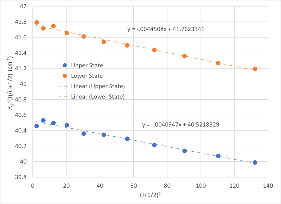
A plot of \(\Delta_2F_J/(J+1/2)\) versus \((J+1/2)^2\) is linear. From the fit:
- the intercept gives \(4B - 6D\),
- the slope gives \(-8D\).
Performing this analysis separately for combination differences that isolate the lower state and the upper state yields \(B''\), \(D''\), \(B'\), and \(D'\).
Vibration–rotation interaction
The rotational constant is not strictly the same for all vibrational states. As a molecule vibrates, the average bond length increases with vibrational excitation, which in turn increases the moment of inertia and reduces the rotational constant.
This effect is described by the vibration–rotation interaction, and the rotational constant in a given vibrational state \(v\) is written as
\[ B_v = B_e - \alpha_e\left(v+\frac{1}{2}\right), \]
where:
- \(B_e\) is the equilibrium rotational constant, corresponding to the bond length at the minimum of the potential energy curve,
- \(\alpha_e\) is the vibration–rotation interaction constant, which quantifies how strongly rotation and vibration are coupled.
For the HCl \(v=1\leftarrow0\) band, the rotational constants \(B''\) (lower state) and \(B'\) (upper state) obtained from combination differences can be used directly to determine \(B_e\) and \(\alpha_e\).
The decrease from \(B''\) to \(B'\) reflects the fact that the bond is, on average, longer in the excited vibrational state.
Big idea: rotation–vibration spectra reveal not only rotational structure, but also how molecular bond lengths change with vibrational excitation through the vibration–rotation interaction.
These constants reveal how the bond length and centrifugal distortion change upon vibrational excitation.
Analyzing the 1-0 Band of HCl near 2990 cm-1
Using the data from Herzberg (ref), shown below, we can construct a table to conveniently plot the Combination Differences:
| J | Line position \((\text{cm}^{-1})\) | Combination differences \(R(J)-P(J)\) | \(\dfrac{\Delta_2 F_J}{J+1/2}\) | \((J+0.5)^2\) | |||
|---|---|---|---|---|---|---|---|
| R-branch | P-branch | Upper | Lower | Upper | Lower | ||
| 0 | 2906.25 | ||||||
| 1 | 2925.78 | 2865.09 | 60.69 | 62.69 | 40.460 | 41.793 | 2.25 |
| 2 | 2944.89 | 2843.56 | 101.33 | 104.29 | 40.532 | 41.716 | 6.25 |
| 3 | 2963.24 | 2821.49 | 141.75 | 146.11 | 40.500 | 41.746 | 12.25 |
| 4 | 2980.90 | 2798.78 | 182.12 | 187.45 | 40.471 | 41.656 | 20.25 |
| 5 | 2997.78 | 2775.79 | 221.99 | 228.87 | 40.362 | 41.613 | 30.25 |
| 6 | 3014.29 | 2752.03 | 262.26 | 270.03 | 40.348 | 41.543 | 42.25 |
| 7 | 3029.96 | 2727.75 | 302.21 | 311.23 | 40.295 | 41.497 | 56.25 |
| 8 | 3044.88 | 2703.06 | 341.82 | 352.23 | 40.214 | 41.439 | 72.25 |
| 9 | 3059.07 | 2677.73 | 381.34 | 392.91 | 40.141 | 41.359 | 90.25 |
| 10 | 3072.76 | 2651.97 | 420.79 | 433.33 | 40.075 | 41.270 | 110.25 |
| 11 | 3085.62 | 2625.74 | 459.88 | 473.76 | 39.990 | 41.197 | 132.25 |
| 12 | 2599.00 | ||||||
This results in the following values:
| Constant | Value \((\text{cm}^{-1})\) | |
|---|---|---|
| Upper state (\(v=1\)) | Lower state (\(v=0\)) | |
| \(B\) | 10.131 | 10.441 |
| \(D\) | 0.000511 | 0.000139 |
| \(B_e\) | 10.596 | |
| \(\alpha_e\) | 0.310 | |
From these results, one can calculate the equilibrium bond length of the molecule, and (as is always good practice) compare the results to those found in the literature (if they exist.)
Combination Differences is a good "first step" in fitting spectral data. However, since taking differences between experimentally measured values introduces increased uncertainty, it is always best to fit the data directly whereever possible. In this case,
\[ \tilde{\nu} = \big[G_1 - G_0\big] + F'_{J'} - F''_{J''}, \]
would be used, with various models for \(G_v\) and \(F_J\) tested, and the results scrutinized to ensure that the fitted constants have statistical significance.
Big idea: combination differences allow rotational constants for both vibrational states to be extracted cleanly from a rotation–vibration spectrum, turning a complex band into precise structural information.