
Spectroscopic Units
In vibrational spectroscopy, energies are almost always reported using spectroscopic units (wavenumbers, \(\text{cm}^{-1}\)) rather than joules. This choice reflects how vibrational spectra are measured and how naturally molecular vibrations relate to frequency.
Experimentally, vibrational transitions are observed by measuring the frequency or wavelength of absorbed or emitted radiation. Reporting results in wavenumbers provides a direct measure of this frequency:
\[ \tilde{\nu} = \frac{1}{\lambda} = \frac{\nu}{c}. \]
Because energy is related to frequency by \(E = h\nu\), using \(\text{cm}^{-1}\) is equivalent to dividing all energies by \(hc\). This produces numbers that are more convenient in size and directly comparable to measured spectra.
Vibrational term values
Instead of working with energies \(E_v\), vibrational levels are often expressed as term values, denoted \(G_v\), defined by
\[ G_v \equiv \frac{E_v}{hc}. \]
For the harmonic oscillator, this gives
\[ G_v = \omega_e\left(v + \frac{1}{2}\right), \]
where \(v = 0,1,2,\ldots\) is the vibrational quantum number and \(\omega_e\) is the harmonic vibrational constant, expressed in \(\text{cm}^{-1}\).
The vibrational constant \(\omega_e\) is related to the molecular force constant and reduced mass by
\[ \omega_e = \frac{1}{2\pi c} \sqrt{\frac{k}{\mu}}. \]
Writing vibrational energies in this form emphasizes that adjacent vibrational levels are equally spaced in the harmonic approximation and that their spacing is directly related to the strength of the bond (\(k\)) and the reduced mass (\( \mu \)).
From this point forward, vibrational energies and transitions will be described using term values \(G_v\) and wavenumbers \(\text{cm}^{-1}\), which is the natural language of vibrational spectroscopy.
Big idea: spectroscopic units connect theory directly to experiment, allowing vibrational energy levels and transition frequencies to be discussed using the quantities that are actually measured.
Worked example: force constant of HBr from \( \omega_e \)
For a diatomic harmonic oscillator, the vibrational term-value constant is \( \omega_e = \frac{1}{2\pi c}\sqrt{\frac{k}{\mu}} \), so we can solve for the force constant: \( k = (2\pi c\,\omega_e)^2\,\mu \).
For HBr, use \( \omega_e = 2648.975\ \text{cm}^{-1} \). :contentReference[oaicite:0]{index=0}
- Convert \( \omega_e \) to SI (m−1): \( 2648.975\ \text{cm}^{-1} = 2.648975\times 10^5\ \text{m}^{-1} \).
- Compute the reduced mass (using isotopes \( ^1\!H \) and \( ^{79}\!Br \)): \( \mu=\frac{m_H m_{Br}}{m_H+m_{Br}} \approx 1.65\times 10^{-27}\ \text{kg} \).
-
Plug into \( k=(2\pi c\,\omega_e)^2\mu \):
\[ k \approx \big(2\pi(2.9979\times 10^8\ \text{m s}^{-1})(2.648975\times 10^5\ \text{m}^{-1})\big)^2 (1.65\times 10^{-27}\ \text{kg}) \approx 4.11\times 10^2\ \text{N m}^{-1}. \]
Interpretation: \( k \) measures bond “stiffness.” Larger \( k \) means a steeper potential well near \( r_e \) and a higher vibrational frequency.
Comparison table: \( \omega_e \), reduced mass \( \mu \), and force constant \( k \)
Force constants computed from \( k=(2\pi c\,\omega_e)^2\mu \). (Reduced masses below were calculated using common isotopes: \( ^{35}\!Cl \), \( ^{79}\!Br \), \( ^{127}\!I \), \( ^{19}\!F \), \( ^{16}\!O \), \( ^{14}\!N \).)
| Molecule | \( \omega_e \) (cm−1) | \( \mu \) (kg) | \( k \) (N/m) |
|---|---|---|---|
| HCl | 2990.95 | 1.63×10⁻²⁷ | 5.16×10² |
| HBr | 2648.975 | 1.65×10⁻²⁷ | 4.11×10² |
| HI | 2309.01 | 1.66×10⁻²⁷ | 3.14×10² |
| F2 | 916.64 | 1.58×10⁻²⁶ | 4.70×10² |
| O2 | 1580 | 1.33×10⁻²⁶ | 1.18×10³ |
| N2 | 2359 | 1.16×10⁻²⁶ | 2.30×10³ |
Source notes for \( \omega_e \): HCl and the O2/N2 values are given in the Oxford notes, while HBr, HI, and F2 are from the NIST Webbook of Chemistry “Constants of Diatomic Molecules” tables.
Although the harmonic oscillator provides a powerful and simple model for molecular vibrations, it has important physical shortcomings. These limitations become apparent when we consider large-amplitude vibrations.
Shortcomings of the harmonic oscillator model
- No molecular dissociation: The harmonic potential \(U(x)=\tfrac{1}{2}kx^2\) increases without bound as \(|x|\rightarrow\infty\). As a result, the model predicts that an infinite amount of energy is required to break a bond, which is not physically realistic.
- Unphysical bond lengths: Because the harmonic potential is symmetric about \(x=0\), it allows the bond to be compressed arbitrarily. In extreme cases, this corresponds to zero or even negative bond lengths, which are not physically meaningful.
These issues indicate that the harmonic oscillator is best viewed as a small-amplitude approximation to real molecular vibrations.
The Morse potential
A more realistic model of a diatomic bond is provided by the Morse potential:
\[ U(x)=D_e\left(1-e^{-\beta x}\right)^2. \]
Here \(D_e\) is the dissociation energy (the depth of the potential well), and \(\beta\) controls the width and steepness of the potential.
Unlike the harmonic potential, the Morse potential:
- approaches a finite energy \(D_e\) as \(x\rightarrow\infty\), allowing for molecular dissociation,
- rises steeply at small bond lengths, preventing unphysical compression.
Anharmonicity and vibrational energy levels
The Morse potential introduces anharmonicity, meaning that the vibrational energy levels are no longer equally spaced. Instead, the term values are well approximated by
\[ G_v = \omega_e\left(v+\frac{1}{2}\right) - \omega_e x_e\left(v+\frac{1}{2}\right)^2. \]
The anharmonicity constant \(x_e\) causes the spacing between adjacent vibrational levels to decrease as \(v\) increases, eventually leading to dissociation.
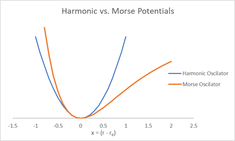
The Morse potential improves on the picture by allowing for dissociation at long bond distances, but still fail at very short bond distances. However, because the Morse potential rises much more quickly as the bond gets shorter, this is less of a problem than with the Harmonic Oscillator.
Big idea: the Morse potential corrects the most serious physical deficiencies of the harmonic oscillator by allowing dissociation and introducing anharmonicity, bringing the vibrational model closer to real molecular behavior.